Skew-T primer
- Bolder Adventures
- Dec 22, 2022
- 5 min read

Many pilots, even experienced ones, are intimidated or overwhelmed by skew-t diagrams. This is unfortunate because besides being probably the most important part of a free-flight forecast, they aren’t nearly as complicated as they appear at first glance. With some background knowledge and a little practice, you can have a very good idea of what to expect from a day from just glancing at the skew-t for less than a minute. I am going to present a crash-course on how to identify some of the most important parameters. You do not need to use any equations or even numbers at all to glean most of the information from a skew-T, once you understand the underlying concepts of stability, it really becomes much more about pattern recognition and applying those basic rules from physics.
First, a brief introduction to the lines and what they mean. Don’t worry about memorizing these lines right now, they are mostly here for reference to make easy visual comparisons of slope. The lines A-E are ordered roughly in terms of descending importance. If all you look at are lines A and B and completely ignore everything else you can get pretty far in understanding how to read a Skew T:
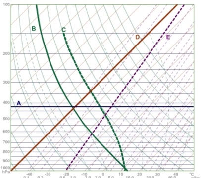
Isobars - These are lines of constant pressure. Because air pressure decreases with altitude, pressure is a good substitute for altitude. If it helps keep the concepts more intuitive, you can safely consider pressure to be interchangeable with altitude. 1000mb is equivalent to sea level, 800mb is equivalent to about 6000’ MSL, 700 mb is about 10,000’, 600mb is about 14,000’ and 500mb is about 18,000’. The actual altitudes vary somewhat with different pressure systems and temperatures, but these approximations are good enough for casual use.
Dry Adiabats - These are the same dry adiabatic lapse rate lines that you should already be familiar with from the concept of stability. The one new piece of information is that the DALR isn’t actually exactly a line. Up to about 18,000’ a line is a good approximation, but at higher altitudes where the air pressure begins to drop asymptotically the DALR takes on more of a curved shape. Fortunately as soaring pilots we really only care about the first 18,000’ or so, so for all intents and purposes you can still think of the DALR as a line.
Saturated Adiabats - These serve a similar purpose to the DALR, but represent the lapse rate of condensing air (i.e. a thermal above cloudbase). They are most useful for seeing how tall a cloud can develop.
Isotherms - These are lines of constant temperature and serve as the X axis. What is a bit different from a traditional graph is that these lines are not perpendicular like a typical x-axis normally is, but instead is rotated 45 degrees, hence the origin of “skew”. These lines are skewed to make some visual analysis easier. Don’t worry about this too much, you can still think of temperature as being on the normal X axis and all the concepts will still work.
Saturated mixing lines - These lines describe how the dewpoint temperature changes as a function of altitude. Notice that these are nearly parallel to the Isotherms. This means that dewpoint only changes slightly with altitude (the dewpoint becomes colder at higher altitudes/lower pressures). This line is most useful to help determine when a given airmass with some variable amount of humidity will condense and form a cloud.
Don’t stress too much about these lines, they are all just used for reference to put the data that is actually plotted into context. They are essentially glorified gridlines and exist for visual reference.
Twice a day every day, weather balloons are launched across the world, 92 of which happen in the United States alone. Each balloon is equipped with an instrument package called a radiosonde which measures pressure, temperature, dew point, and GPS location and radios that data back to the ground. Using this data meteorologists are able to map the atmosphere which is one of the most important parameters driving the forecast models. This is just one example of what that data looks like:

The red line should look familiar; it is the ELR. The blue line is the dewpoint. Off to the right the windspeed and direction are displayed as barbed arrows. Further right are a number of calculated parameters. Most of these are not especially useful to soaring pilots and can be largely ignored. The background gridlines are the same as introduced above
Modern apps do a good job of automating skew-t analysis and are a nice way to familiarizing yourself with how these charts work. I will be using the skew-t app from the android store to demonstrate how you can derive some of the most important parameters from a skew-t
1. Top of lift
In order for a thermal to remain buoyant, it must be warmer than the environmental lapse rate at any given altitude. As soon as it reaches the same temperature, it stops rising. We can find at what altitude this occurs by following the dry adiabat from its source at the ground and see where it intersects the ELR.

Thermals must be warmer than their surroundings to have enough buoyancy to release from the ground. Typically they will start 1-3℃ warmer than the average surface temperature. The precise value depends greatly upon how much sun the ground receives, how easily the surface absorbs heat, and how much wind disturbs the warming pool of air. Sunny, dry, and low-wind areas like you find in the high desert tend towards the higher end, while shaded, windy, and wet areas will be near the lower end. In any case, the thermal begins warmer than the ground and if the atmosphere above it is unstable, it will rise. Here we choose a point a few degrees warmer than the ELR at the surface, and follow the dry adiabat upwards which simulates how the thermal cools as it rises. The altitude at which the thermal intersects the ELR defines the absolute top of the thermals.
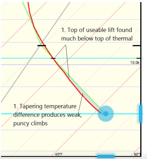
2. Thermal strength

Closely related to the top of lift is how strong thermals actually are. This depends entirely on how much warmer the thermal is than the surrounding air. Large temperature differences generate strong climbs, small temperature differences result in weak climbs. Because gliders have a sink rate of about 200fpm, there is a minimum temperature surplus the thermal must have simply to provide a net zero climb rate for a glider. Because of this, we can rarely actually reach the true top of thermal and in practice the climb will end once the thermal begins to get close to the ELR. The best soaring days are when the ELR is highly unstable and maintains a wide temperature difference for most of the climb. In contrast, thermals which gradually taper off in temperature difference tend to be small and punchy, as the weaker outer edges of the core are left behind and only the small, strongest parts of the core can continue to rise upwards. A less ideal thermal day looks like below.
3. Cloud Base
When a thermal forms, it carries air from the surface up to altitude. For the most part, this air does not mix significantly with the air it rises into, so essentially it retains whatever moisture it started with. This amount of moisture will condense at its dew point, and the dew point changes slightly (colder) as it rises into lower pressure air. We can find how the dewpoint changes with altitude by following the saturated mixing line up from the surface.

In this particular case, the thermal intersects the ELR and stops rising before it cools down enough to cause the moisture it is carrying to condense. Thus, no clouds form.
Comments